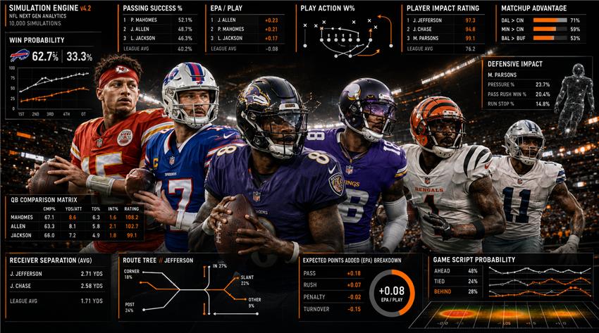
How the New Simulation Works

We give the actual functions the engine uses, walk a snap through them in order - the resolution primitive, play-calling, coverage geometry, the pass-rush clock, the catch, interceptions, pursuit and tackling, the run game, fumbles, and the season Monte Carlo - and quote the real calibration constants where they help. If you want the casual version, this is not it.

Why this beats one offense number against one defense number

The usual shortcut is to rate each team's offense and defense as a single number and pit them against each other. The problem is that aggregation throws away exactly the information that decides games. Football is not 11 average players; it is specific people lined up across from specific people, and the outcome is driven by where the edges and the holes happen to line up. A single rating literally averages those mismatches out of existence.

Because this engine resolves every snap as the actual one-on-one matchups, it surfaces the things a team-level number cannot:

• A great unit with one weak link. A top-five offense whose right tackle is a backup will leak pressure all day against an elite edge rusher, because the pass-rush clock is computed per blocker. A single offense rating shows a juggernaut; the matchup shows the quarterback running for his life on every dropback to that side.
• A star taken away. Put a shadow corner on a number-one receiver and the coverage geometry tightens his window while the target logic moves the ball to lesser options. The offense's overall rating barely moves; its real, on-field efficiency falls off a cliff. A coarse model never sees the ball get redirected.
• Unit-versus-unit edges. An elite run-blocking line against a pass-rush-first front gashes it on the ground, even if both teams look average overall, because the run game weighs run-block grades against that specific front's run-defense grades, not a blended team number.
• Yards that are not points. A secondary that allows catches but tackles them dead gives up yardage without giving up scores, because coverage suppresses yards after the catch independently of completions. A single "yards allowed" or one defensive rating conflates the two; the engine separates them, which is why it can tell a bend-but-don't-break defense from a sieve.
• Same rating, different shape. Two teams that grade out identically on paper can project very differently, because what matters is whether one team's strength is pointed at the other team's weakness. The matchup engine answers that question directly; an overall-versus-overall model assumes it away.

That is the whole pitch: it does not tell you which team is better in the abstract, it tells you where one team has an edge over the other this week, and how often that edge actually shows up on the scoreboard once you account for pace, game script, and a few hundred snaps of variance. The rest of this article is how it does that.

1. The resolution primitive

Almost every contested event resolves through one tiny, stateless math library. There are no linear "0.5 + slope * diff then clamp" formulas anywhere in the new engine - that pattern is exactly what compresses a league onto a flat ceiling and kills the tails. Instead:

Sigmoid and logit.

sigmoid(x) = 1 / (1 + e^(-x)) logit(p) = ln( p / (1 - p) )

Head-to-head win probability for attacker rating a vs defender rating d on the shared grade scale:

WinProbability(a, d, scale) = sigmoid( (a - d) / scale )

The scale is grade-points-per-logit: smaller means talent dominates, larger means more randomness. It is fit so the model's win-rate spread matches real data (default head-to-head scale = 18, which makes a 90-vs-55 mismatch win about 0.87 of the time, versus the old clamped 0.58).

Absolute rate anchored at a baseline (used when the event is a rate nudged by several combined signals rather than a clean one-on-one):

RateFromBaseline(base, delta, K) = sigmoid( logit(base) + delta / K )

where base is the league-neutral rate, delta is the net grade signal, and K is the grade-points-per-logit calibration. Because the shift happens in log-odds and returns through the sigmoid, the output is always a valid probability and never needs clamping.

Yardage is not a bounded draw with a bolted-on big-play slot. It is sampled from a heavy-tailed lognormal whose median and spread move with the matchup:

z ~ N(0,1) // Box-Muller from two uniforms yards = median * e^(logSd * z) - floor

The high side is intentionally unbounded; the only cap the caller applies is physical (distance to the goal line). Subtracting floor lets a draw go negative so stuffs and losses occur naturally. Where a top end needs taming the engine uses a smooth asymptote, never a hard min:

SoftCap(x, knee, ceiling) = knee + (ceiling - knee) * (1 - e^(-(x - knee)/(ceiling - knee))) for x > knee

The realism dial injects uniform noise into the log-odds (scaled by randomnessLevel / 0.5) before the sigmoid, so a low setting is near-deterministic and a high setting is volatile, without ever leaving (0,1).

2. Grades to standardized signals

Every player carries position-specific performance stats. Before entering a contest each relevant rating is standardized against a league baseline and spread:

z = (grade - baseline) / spread

Representative calibration: quarterback passing baseline / spread = 72.2 / 10.6, accuracy 75.0 / 2.9, receiving 67.6 / 10.4, coverage 62.0 / 9.0. Standardizing means a one-unit edge is the same amount of edge for a rusher, a corner, or a receiver, so blends across positions are apples to apples.

3. Choosing the play

Pass-or-run is a probability built from the offense's real tendency, then adjusted. With league average pass rate L = 0.535 and the team's real base pass rate b:

passTendency = L + (b - L) * (1 + PassRateSpread) // widen team identity around the mean + scriptDelta * GameScriptPassScale // damped scoreboard effect + downDistanceTerms + rbOveruseTerm + adjust passTendency = clamp(passTendency, 0.12, 0.88) chosePass = rand() < passTendency

scriptDelta accumulates the game-script swings (for example a fourth-quarter deficit of 17+ adds about +0.16, a three-score lead subtracts up to about -0.55), then is scaled by GameScriptPassScale = 0.35. It is damped on purpose: a team's real base rate already encodes some script, and running the scoreboard at full strength made trailing teams pass far too much (sim pass-rate-vs-wins correlation went to -0.64). Down and distance stay at full strength (third-and-long about +0.15, short yardage about -0.12). Kneels, spikes, the trailing-and-late Hail Mary, and a dedicated fourth-down decision short-circuit the draw. The defense then reads the formation (play-action counts as run) and picks scheme plus personnel.

4. Alignment

The 22 players are placed on a coordinate field by offensive personnel and the defensive shell (press or off, one-high or two-high). Receivers get routes that break at real depths. From here, distances are literal: nearest defender to a catch point, who is play-side on a run, how much separation a route earned.

5. Coverage geometry

At the throw frame, each route runner is paired with the nearest man defender, who is placed trailing him by a cushion set by the matchup:

cushion = SeparationBase + (recvGrade - covGrade) * SeparationScale + noise - DefenseCoverageInfluence * max(0, covGrade - 60) // asymmetric: only good corners squeeze cushion = max(cushion, SeparationFloor)

with SeparationBase = 1.8 yds, SeparationScale = 0.06 yds per grade point, SeparationFloor = 0.3, DefenseCoverageInfluence = 0.062. The tightening is one-sided so elite coverage suppresses completions and YAC without symmetrically over-opening receivers against weak corners. After positioning, a receiver's separation is simply the Euclidean distance to the nearest able defender.

Zone defenders are not static landmarks. Each drives a fraction of the way toward the nearest receiver before separation is measured:

frac = ZoneBreakWeight * (0.5 + (covGrade - 55) / 70), clamped to [0, 0.9] d.pos += (receiver.pos - d.pos) * frac

so a better zone defender (higher coverage grade) closes harder, but the cap below 1.0 always leaves a throwing window. Bracket coverage pulls the deepest safety over a flagged receiver - either a true star by grade, or one who has drawn an outsized in-game target share - which both tightens his window and vacates the safety's deep zone, so a deep route elsewhere genuinely opens up.

6. The pass-rush clock

Each rusher is resolved against his assigned blocker. With gradeDiff = (rusherGrade - blockerGrade) * PassRushGradeSpread (the spread term mildly compresses the gap so elite rushers do not monopolize sacks):

winProb = sigmoid( gradeDiff / WinLogisticScale ) // free rushers add a logit bonus if win: tw = sigmoid( gradeDiff / TimeLogisticScale ) timeToWin = (BaseTimeToWin + TimeRange) - TimeRange * tw

So a big mismatch saturates tw toward 1 and the rusher arrives near BaseTimeToWin; an even rep arrives near BaseTimeToWin + TimeRange. Free rushers win fast (a fixed short time plus jitter); reactive blitz-pickup blocks by backs and tight ends are penalized and floored. The earliest winning rusher sets when pressure arrives.

7. Time to throw, and stepping the frame

The quarterback's release races that clock. With his real average time to throw ttt and the pocket time pocket from the rush:

ForcedThrow: tThrow = ttt - PressureTimeWeight * (ttt - pocket) (if pocket < ttt) EscapedAndThrew: tThrow = ttt + ScrambleTimeBonus Clean: tThrow = ttt + CleanPocketTimeBonus * (pocket - ttt) (if pocket > ttt) tThrow = clamp(tThrow, 1.2, 4.0)

Receivers are advanced to exactly tThrow, so a hurried throw catches them shallow and less separated. Then man coverage, bracket, and zone-break are applied in that order, and separation is measured.

8. Target selection

A grade-weighted default target is the seed, then realistic redistributions fire probabilistically: a route-aware redirect to whoever is open on this play's routes; a deep-ball spread that moves a deep shot off the number-one receiver to another deep man; a red-zone tight-end lever; and a covered-checkdown that completes to an open outlet instead of forcing a blanketed short route. These keep target and yardage distributions realistic instead of funneling everything to WR1.

9. Air yards

Credited air yards take the receiver's route depth and scale it multiplicatively by the passer's average depth of target relative to the league mean:

qbDepthFactor = 1 + PassDepthQbShare * ((qbADOT - QbAdotMean) / QbAdotMean), floored at 0.4 airYards = routeDepth * qbDepthFactor * AirYardsScale

with QbAdotMean = 8.32, PassDepthQbShare = 1.3, AirYardsScale = 0.91. Multiplicative (not additive) scaling preserves each receiver's depth differentiation while a checkdown-heavy passer shortens all of his throws proportionally, lowering his yards per attempt without flattening his receivers.

10. The catch contest

Completion is a player-stat contest, not geometry. Build standardized halves:

qbZ = (1 - QbCompletionGradeShare)*accZ + QbCompletionGradeShare*gradeZ // QbCompletionGradeShare = 0.85 recZ = (recvGrade - RecGradeBaseline) / RecGradeSpread dbZ = (covGrade - CovGradeBaseline) / CovGradeSpread (+ bracket term if a 2nd defender is within radius) offenseSignal = QbReceiverSplit*qbZ + (1 - QbReceiverSplit)*recZ // QbReceiverSplit = 0.60 balanced = offenseSignal - dbZ shift = CompletionSpread * balanced (+ depth, position, pressure, double-coverage terms)

The base rate is depth-banded (short < 8 air yds, medium 8 to 18, deep > 18) and a strong cover man lowers the effective base (so an elite receiver cannot saturate against a real corner). Then:

completeProb = RateFromBaseline(effBase, shift, CompletionPointsPerLogit)

The quarterback is deliberately the larger share of the offense signal (60 percent), so a poor passer cannot post elite numbers behind open receivers. Position terms lift tight ends and backs and trim receivers to match real target-share-vs-catch-rate; a duress throw and a heavily double-covered man subtract from the shift.

11. Anchoring to real efficiency

The contest output is then blended toward the specific player's real rate. Each anchor is a convex blend:

p' = (1 - anchor) * p + anchor * realRate

Applied for the receiver's real catch rate (receivers anchored harder than tight ends and backs, who legitimately catch a high share), the quarterback's real completion percentage, his yards per completion (on the yardage, see below), and, on throws that can reach the end zone, his real touchdown rate. The touchdown anchor is asymmetric: it only pulls down quarterbacks converting below their real red-zone rate, so it corrects poor finishers without inflating good ones. This is the backbone that keeps season stat lines true while the matchups supply variance, spread, and opponent effects.

12. Interceptions

Two independent paths. First, a centerfield robber: before the catch, a deep safety reading the quarterback can break on a middle throw meant for someone else, with probability scaled by his ball skill, the passer's turnover-worthy rate, and throw depth. Second, the target-vicinity pick:

intChance = twp * (0.5 + tightness) * InterceptionRateAdjust * intGradeFactor * convFactor * covPosFactor intGradeFactor = max(0.1, 1 - PassIntGradeWeight * gradeZ) convFactor = (ballSkill / IntConversionSkillRef) ^ IntConversionSkillWeight covPosFactor = per-position propensity of the covering defender (DB 1.0, LB 0.15, DL 0.20)

where twp is the quarterback's turnover-worthy-throw rate and tightness comes from the cover defender's coverage grade. The conversion factor and position factor are why a ball-hawk safety turns a tight window into a pick far more than an underneath linebacker, and a tunable share (currently 0.40) of would-be linebacker picks are reattributed as tipped balls to the line. Together these land the realistic DB / LB / DL split (about 74 / 17 / 9) instead of over-crediting underneath defenders.

13. Pursuit and tackling geometry

Yards after the catch and all run yards share one pursuit model. The carrier runs the line x = carrierX from carrierY upfield at speed cs. A defender at (dx, dy) with effective speed dse = defSpeed * 0.92 (the 0.92 is reaction and angle loss) can make a play if there is a time t in (0, 4.5] solving:

|defender - carrier(t)| <= dse * t => (cs^2 - dse^2) t^2 + 2 (cy - dy) cs * t + |defender - carrier|^2 <= 0

The smallest valid root gives the intercept depth InterceptY = carrierY + cs * t. Defenders who cannot solve it within the horizon (bad angle, too far, backside pursuit on a forward-moving carrier) never enter the contest at all - which is how a sweep faces only play-side defenders. The reachable defenders are sorted by intercept depth and contested in order:

breakProb = RateFromBaseline(BreakBaselineRate, carrierBreak - defenderTackle, BreakSensitivity) + noise

with BreakBaselineRate = 0.09 and BreakSensitivity = 32. A broken tackle removes that defender and the run continues to the next intercept point; beating everyone to the goal is a touchdown. Note there is no clamp to the start line, so a penetrating defender intercepts behind the line for a tackle for loss. Finally, contact-point variance scatters the spot (a tackle is not a point event):

g ~ approx N(0,1) (sum of three uniforms); finalY += g * RunContactSpread // RunContactSpread = 2.4

For YAC, the same model runs with a higher break baseline and a coverage-suppression term subtracted from the delta, so a cover man in phase at the catch tackles immediately:

delta = receiverYac - defenderTackle - CoverageYacSuppression * covZ // CoverageYacSuppression = 5.5

14. The run play

Blocking is resolved per pair (offensive line vs front, plus a climb block on the play-side linebacker) with the same win-probability logistic; losers are engaged, winners penetrate. A deep safety fills the alley on a share of plays. The back starts at the mesh point on his lateral track and the pursuit geometry above produces a raw gain, which is then anchored toward his real efficiency:

total = (1 - w) * geometryYards + w * realYpc // w = RushEfficiencyWeight = 0.5 // QB designed runs use w >= 0.75 (open-field scrambles the interior geometry can't reconstruct); // QB sneaks are exempt and stay short. total += RunBlockYardsWeight * (((olRunBlock - dlRunDefense) - RunBlockMatchupCenter) / RunBlockMatchupSpread)

with RbYpcBaseline = 4.30, RunBlockYardsWeight = 0.8, RunBlockMatchupCenter = 8.5 (it removes the systematic league-wide gap, since the defenders who rush on run downs grade low vs the run, so only a genuine blocking edge gains yards), RunBlockMatchupSpread = 10. Inside the ten, a goal-line stand stuffs a share of would-be scores; there is no positive yardage floor (a stuffed run loses what the geometry says), bounded only by the back's own goal line, which scores as a safety.

15. Fumbles

Fumbles are a separate, completion-neutral turnover lever (so tuning them does not disturb passing efficiency). Per exposed touch:

fumbleRate = BaseFumbleRate * (1 + (60 - ballSecurityGrade) / FumbleGradeScaleDivisor) * positionMultiplier // inside catch 1.25, sideline catch 0.75 * randomnessScale fumbleRate = clamp(fumbleRate, FumbleRateCapMin, FumbleRateCapMax)

with BaseFumbleRate = 0.035 (targeting about 1.0 lost fumble per team per game). The forcer is the tackler on the play; recovery is then resolved, and a defensive recovery can be returned (a scoop-and-score is a live outcome). Field goals, extra points, punts, kneels, spikes, incompletions and interceptions are exempt from the fumble check.

16. Special teams and the drive loop

Field goals and extra points succeed as a function of distance and kicker reliability; punts flip field position with placement and touchback handling; returns produce realistic yardage with a live, small return-touchdown chance. Plays chain into drives: down and distance update from yardage, first downs reset the chains, scores and turnovers end possessions, and the clock runs realistic time per play with each team's real plays-per-game pace folded in. Quarter, half, two-minute and overtime state all feed back into the play-caller, so hurry-up, clock-killing, and kneel-downs emerge rather than being scripted.

17. Setting a player's level: injury years and aging

A grade reflects how a player performed in the season it was earned, so projecting him to a future season takes two steps: establish his true current level, then move it along his career arc.

Current level (small-sample / injury anchoring). A grade is a per-snap rate, so an injury-shortened season is not deflated by low volume, but it is noisy - grades only stabilize over a few hundred snaps. A small sample is therefore regressed, but toward the player's OWN most recent full season rather than toward league average:

blended = g_current * conf + g_priorFullSeason * (1 - conf), conf = snaps / threshold

This is empirical-Bayes toward self: a star who played three games anchors to his established level, not to a replacement-level 50, while a genuine one-year sample with no track record still regresses toward a modest prior. Volume is handled separately by the snap allocator, which already regresses a low-games starter back toward a full starter's share, so an injured starter still plays a full projected season. The upshot is that a player who has genuinely declined shows it (his recent grades are lower), but a player who merely got hurt is not mistaken for an average one.

Career arc (the age curve). Every player is then moved along a generic, position-specific age curve - a development rise, a flat prime plateau, then decline (gentle at first, with a steeper late cliff for the positions that fall off hard, such as running backs and corners). It is applied as a FORWARD delta from the age at which the grade was earned to the simulated season's age:

delta = Level(projectionAge) - Level(statYearAge)

where Level() is 0 across the plateau and negative on either side. A same-age call - a historical or cross-era replay using that year's grade - returns 0, so replays stay faithful; only forward projections age. The rise is ceiling-aware so an already-elite young player is not pushed past a realistic maximum: the development bump fades to zero as a grade nears the ceiling.

room = clamp((97 - grade) / 9, 0, 1); riseDelta *= room // decline is left intact

Efficiency rates (completion %, yards per attempt, catch rate, and the rest) move proportionally with the same age delta, and the curve is league-neutral - it redistributes between rising youth and aging veterans without shifting league-average grade. Net effect: a young ascender climbs, a prime player holds, an aging great fades, and an injured star reads as his real self instead of a three-game fluke.

18. From one game to a projection

A single game is one draw. A season projection is a Monte Carlo: run the full schedule N times and average. Standings, Super Bowl and playoff odds, team stats and player leaders are the expectation across the runs. Because the seasons are independent draws, the standard error of every projected average falls like 1 / sqrt(N) - so more simulations mean tighter, more trustworthy numbers, which is the whole reason a 100-season projection is steadier than a 10-season one.

A note on the constants

The numbers above are current calibration values. Probability scales are fit so the model's spreads match real distributions, and the efficiency anchors and baselines are tuned against real league and per-player data, then re-checked whenever the engine changes. They are levers, not laws - but every one of them moves a likelihood or a piece of geometry. Nothing in the engine is a hard cap.

What you can do with it

Put two teams in and you are not getting a vibe or a power-ranking gap. You are getting the product of every matchup on the field: where one side can win up front, which receiver gets taken away and where the ball goes instead, whose ground game travels against whose front, and how all of that compounds across a few hundred snaps once pace and game script are folded in. That is what lets it flag an upset a rating model calls a blowout, or expose a contender whose one soft spot happens to sit across from the league's best at attacking it. Run a single matchup, or simulate a full season hundreds of times and read the edges off the averages. Either way, it is answering the only question that matters: not who is better on paper, but who has the edge in this game, and how often it holds up.